
An introduction to loiccoyle/phomo.
The docs are available here.
The shoulders on which I stand
Photo mosaics are images composed of many smaller images arranged to best reconstruct the master image. The details of the smaller images are visible up close but blur and blend into the master image as the magnification decreases.
I’ll refer the big image as the master image and small images as the tile images.

There already exists a couple great photo mosaic python libraries:
Both these projects arrange the tile images by dividing the master image into smaller regions, computing the average colours of the tiles and regions and then assigning the tile with the closest average colour to the region.
While this method is very computationally efficient, by using the average colour, it loses a lot of the information contained in the tiles and master regions. This can lead loss of detail and suboptimal assignments.
With this said, the goal of phomo is to extend on the current photo mosaic libraries mainly improving the tile assignment algorithm and squeezing out more performance.
Features
The main features of phomo are:
- improved tile to master region metric
- optimal tile assignment algorithm
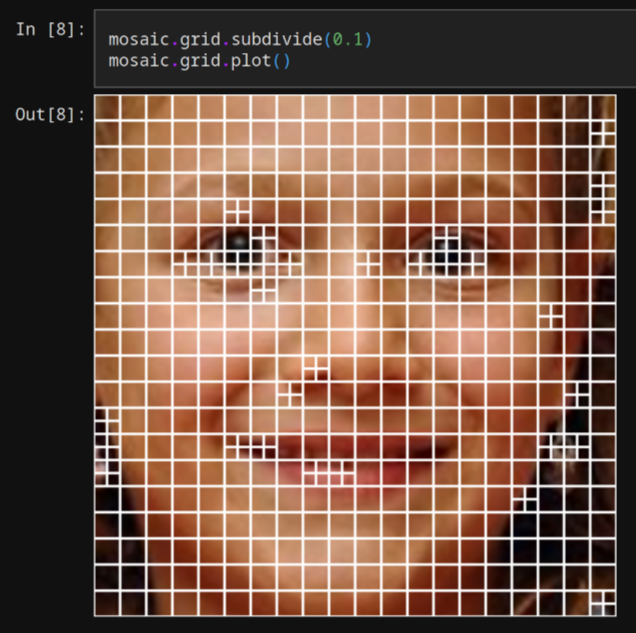
- master region grid visualization and subdivision
- colour palette matching
- concurrent computation & GPU acceleration
Tile to master region loss metric
Instead of using the average colour differences as the deciding metric in the tile assignment algorithm, why not use the difference of the colour distribution of the tile images and the master regions.
To illustrate the advantages of this method compared to the average colour metric, let us consider a single high contract master region.
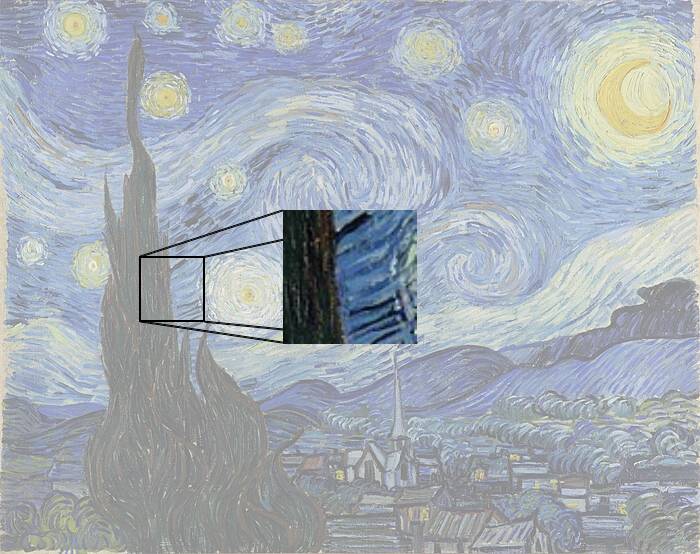
And let us assume that we want to decide which of the following two tiles to assign to the master region.

The tile on the left contains the average colour of the master region, and the tile on the right is a picture of a cypress tree in front of a blue sky.
When using the average colour difference metric, the assignment algorithm would favour the tile on the left which would lose the contrast of the master region. By using the full colour distribution difference, the assignment algorithm would favour the tile on the right, which does a better job at preserving the contrast of the master region.
phomoactually implements a few different metrics which all make use of the spatial distribution of the colours within the tiles and master regions. The effect of the different metrics is showcased in the metrics example.
Tile assignment algorithm
Great, so we have a nice way of measuring the compatibility of the tiles with the master regions, but now comes the question of using this metric to figure out which tile goes where. Let us assume we have computed the loss metric between every tile and master region and stored the results in a matrix.
This matrix is referred to as the distance matrix.
The goal is the assign each tile to a master region while minimizing the loss over the entire reconstructed mosaic.
This is a well known problem, referred to as the assignment problem, which luckily for me has a well known solution: the Hungarian algorithm, a variant of which is implemented in scipy as scipy.optimize.linear_sum_assignment.
Master region grid
When exploring existing libraries, I quite liked the grid visualization and subdivision features of the danielballan/photomosaic package, showcased in their docs. The basic idea is to subdivide master regions with high contrast into smaller regions, effectively increasing the resolution in these high contrast regions.
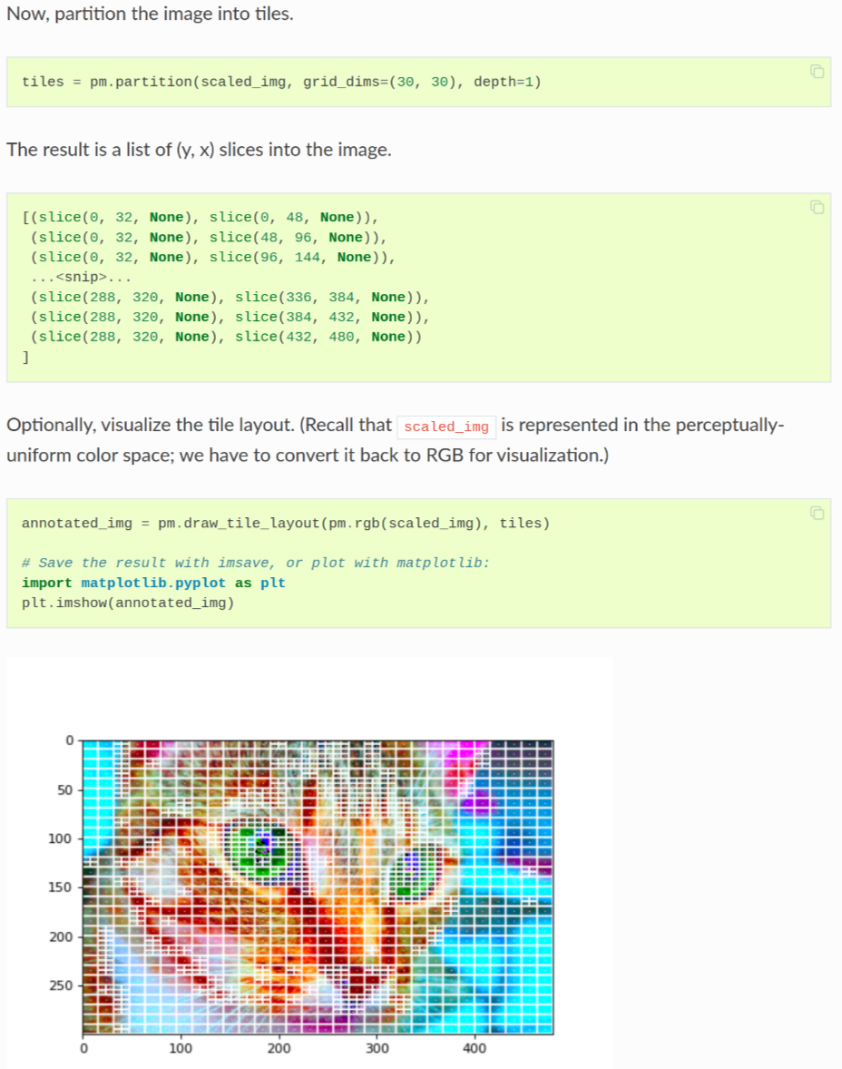
As such this feature was implemented in phomo and an example of its usage is shown in the faces example.
Colour palette matching
This feature is inspired by the palette adjustment feature in danielballan/photomosaic.
To create good looking photo mosaics, it helps to have similar colour distributions between the master regions and the tiles.
Assume we have a master image with a blue colour palette and our tiles are mostly reddish, then we obviously won’t obtain the most accurate photomosaic.
phomo provides three methods to match the tile and master image colour palettes.
- palette normalisation: This method stretches out the colour distributions of both the tiles and the master images to cover the full colour space, this will lead to more appealing photo mosaics but will sacrifice the fidelity of both the master and tile images.
- match the tile images to the master image: This method uses the Reinhard colour transfer algorithm to transfer the colour distribution of the master image to the tiles. This will leave the master image unchanged but will alter the tile images.
- match the master image to the tile images: Similar to the previous method, this uses the same colour transfer algorithm to transger the colour distribution of the tiles to the master image. This will leave the tile images unchanged but will alter the master image.
These three methods are showcased in the colour matching example.
Concurrent computation
phomo has a few tricks to improve the computation speed of the distance matrix. The simplest of which is to leverage the user’s multiple cores parallelize the computation. Each worker is given a chunk of the tile images and computes the loss metric between its tiles and the master regions. The workers then combine their results to produce the distance matrix.
An alternative method to speed up the distance metric computation is to use the GPU to accelerate the computation. phomo provides a CUDA kernel which computes the loss metric on the GPU. This requires the user to have a compatible GPU as well as enough VRAM to store the master regions and tiles. phomo uses the numba library to compile python code to CUDA kernels. This method significantly speeds up the distance matrix computation.
...
@cuda.jit
def compute_d_matrix_kernel(master_arrays, pool_arrays, d_matrix):
    i, j = cuda.grid(2)  # type: ignore
    if i < master_arrays.shape[0] and j < pool_arrays.shape[0]:
        distance = 0.0
        for x in range(master_arrays.shape[1]):
            for y in range(master_arrays.shape[2]):
                for c in range(master_arrays.shape[3]):
                    diff = master_arrays[i, x, y, c] - pool_arrays[j, x, y, c]
                    distance += diff * diff
        d_matrix[i, j] = math.sqrt(distance)
...
An example showcasing these two methods is provided in the performance example. On my system, GPU acceleration leads to a 30x speed increase.